
There are currently two models to choose from.
- Predict how water moves through your Area of Interest.
- Predict the water quality of the runoff from your Area of Interest.
7.1 Site Storm Model
The Model My Watershed Site Storm Model simulates a single 24-hour storm by applying a hybrid of the Source Loading and Management Model (SLAMM), TR-55, and the simplest of the Food and Agriculture Organization of the United Nations evaporation models for runoff quantity and EPA’s STEP-L model for water quality over the selected Area of Interest.
The results are calculated based on actual land cover data (from the USGS National Land Cover Database 2011, NLCD2011) and actual soil data (from the USDA Gridded Soil Survey Geographic Database, gSSURGO, 2016) for the selected land area of interest. For more information and data sources, refer to Section 3.2, Coverage Grids.
Learn how to use the Site Storm Model in Model My Watershed.
7.1.1 TR-55 Component
This model is used to calculate runoff for all “natural” land-use types. TR-55 curve number information
7.1.2 SLAMM Component
The Source Loading and Management Model (SLAMM) is used to calculate runoff for urban land-use types.
7.2 Watershed Multi-Year Model
The Watershed Multi-Year Model in Model My Watershed simulates 30 years of daily water, nutrient, and sediment fluxes using the Generalized Watershed Loading Function Enhanced (GWLF-E) model, developed for the MapShed desktop modeling application by Barry M. Evans, Ph.D., and his group at Penn State University. The GWLF-E model is also one of five watershed models available within EPA’s BASINS multi-purpose modeling application.
Model My Watershed is now the primary framework for running the latest GWLF-E model version, replacing MapShed and BASINS, as these two desktop applications are built on the aging MapWindow GIS package, which is no longer supported. For that reason, in late 2014, we ported all GWLF-E code from Visual Basic to Python, and all subsequent development has been in this open source repository. Similarly, all MapWindow-based geoprocessing routines have been rewritten to operate with the open-source GeoTrellis geographic data processing engine and framework, with all new code located in this repository.
7.2.1 The GWLF Model
The core watershed multi-year simulation model used in MMW and MapShed (GWLF-E) is an enhanced version of the Generalized Watershed Loading Function (GWLF) model first developed by researchers at Cornell University (Haith and Shoemaker, 1987). The original DOS-compatible version of GWLF was rewritten in Visual Basic by Evans et al. (2002) to facilitate integration with ArcView© and other GIS software packages, and tested extensively in the U.S. and elsewhere. Since 2002, it has been substantially enhanced; see Section 7.2.2 GWLF-Enhancements.
The advantage of GWLF (and GWLF-E) is its ease of use and reliance on input datasets that are less complex than those required by other watershed-oriented water-quality models such as SWAT, SWMM, and HSPF (Deliman et al., 1999). The U.S. EPA has also endorsed the model as a good “mid-level” model that contains algorithms for simulating most of the key mechanisms controlling nutrient and sediment fluxes within a watershed (U.S. EPA, 1999).
The GWLF model can simulate runoff, sediment, and nutrient (nitrogen and phosphorus) loads from a watershed, accounting for variable-size source areas (e.g., agricultural, forested, and developed land). It also includes algorithms for calculating septic system loads and allows the inclusion of point-source discharge data. It is a continuous simulation model that uses daily time steps for weather data and water balance calculations. Monthly calculations of sediment and nutrient loads are based on the daily water balance accumulated to monthly totals.
GWLF is considered a combined distributed and lumped-parameter watershed model. For surface loading, it is distributed, allowing multiple land-use/cover scenarios. Still, each area is assumed to be homogeneous with respect to the various landscape attributes considered by the model. Additionally, the model does not spatially distribute the source areas, but aggregates the loads from each source area into a watershed total; in other words, there is no spatial routing.
For subsurface loading, the model operates as a lumped-parameter model, utilizing a water balance approach. No distinctly separate areas are considered for sub-surface flow contributions. Daily water balances are computed for an unsaturated zone as well as a saturated subsurface zone, where infiltration is computed as the difference between precipitation and snowmelt minus surface runoff plus evapotranspiration.
For major processes, GWLF simulates surface runoff using the SCS-CN approach with daily weather (temperature and precipitation) inputs from the EPA Center for Exposure Assessment Modeling (CEAM) meteorological data distribution. Erosion and sediment yield are estimated using monthly erosion calculations based on the USLE algorithm (with monthly rainfall-runoff coefficients) and a monthly KLSCP value for each source area (i.e., land cover/soil type combination). A sediment delivery ratio based on watershed size and a transport capacity based on average daily runoff is then applied to the calculated erosion to determine sediment yield for each source area. Surface nutrient losses are determined by applying dissolved N and P coefficients to surface runoff and a sediment coefficient to the yield portion for each agricultural source area.
Point source discharges can also contribute to dissolved losses and are specified in terms of kilograms per month. Manured areas and septic systems can also be considered. Urban nutrient inputs are assumed to be in the solid phase, and the model uses an exponential accumulation and wash-off function for these loadings. Subsurface losses are calculated using dissolved N and P coefficients for shallow groundwater contributions to stream nutrient loads, and the subsurface submodel considers only a single, lumped-parameter contributing area.
Evapotranspiration is determined using daily weather data and a cover factor that depends on land use/cover type. Finally, a water balance is performed daily using supplied or computed precipitation, snowmelt, initial unsaturated zone storage, maximum available zone storage, and evapotranspiration values.
It is beyond the scope of this document to provide specific details on the structure and technical components underlying the original GWLF model. View a copy of the GWLF manual. Additional details on the updated version of this model (GWLF-E) and the geoprocessing routines used in MapShed (and, by extension, Model My Watershed) to prepare input data for the model can also be found in the MapShed Users’ Manual, available at this website.
7.2.2 GWLF-Enhanced
Since its initial incorporation into MapShed (and its precursor, AVGWLF), the GWLF-E model has been substantially enhanced, beginning in 2002, to include a number of routines and functions not present in the original GWLF model.
A significant revision in an earlier version of AVGWLF was the inclusion of a streambank-erosion routine. This routine is based on an approach often used in geomorphology, in which monthly streambank erosion is estimated by first calculating a watershed-specific average Lateral Erosion Rate (LER). After a value for LER has been computed, the total sediment load generated via streambank erosion is then calculated by multiplying the above erosion rate by the total length of streams in the watershed (in meters), the average streambank height (in meters), and an average soil bulk density value (in kg/m3).
In Mapshed, these stream bank and erosion rate parameters were optimized for models using the high-resolution stream flow line dataset available for Pennsylvania. In Model My Watershed, which utilizes NHDplus v2 medium-resolution flow lines, we apply a sediment erosion adjustment factor of 1.4 to ensure that bank erosion estimates in Model My Watershed are comparable to those in MapShed for Pennsylvania.
In later versions, the original water balance routine within GWLF was extended to simulate water withdrawals from surface and groundwater sources. Within MapShed, information from an optional “water extraction” GIS layer can be used to estimate the volume of water extracted from various sources within a watershed each month. For surface water withdrawals, the estimated cumulative water volume is subtracted from the simulated “stream flow” component of the monthly water balance calculations. For groundwater withdrawals, this volume is subtracted from the “subsurface” component of the monthly water balance calculations. (Note: This particular routine is not yet implemented in Model My Watershed, although the GWLF-E model does allow for “extracted” water to be simulated.)
Other recent model revisions include the implementation of an agricultural tile drainage routine, the capability to consider point source effluent (i.e., flows) in the hydrology for a given area, the incorporation of new routines for more direct simulation of loads from farm animals, a new pathogen load estimation routine, and the ability to consider the potential effects of best management practices (BMPs) and other mitigation activities on pollutant loads.
Another significant improvement has been in the simulation of hydrology and loads from urban areas. In the original version of GWLF used with AVGWLF, such a simulation could only be accomplished for two basic types of urbanized or developed land (i.e., low-density development and high-density development). However, in very intensively developed watersheds, it may be more appropriate to use more complex routines for a broader range of urban landscape conditions. Consequently, additional modeling routines have been included with the version of GWLF used in MapShed and Model My Watershed to address this situation. These new functions are based on the RUNQUAL model developed by Haith (1993) at Cornell University. With these routines, runoff volumes are calculated from procedures given in the U.S. Soil Conservation Service’s Technical Release 55 (U.S. Soil Conservation Service, 1986). Contaminant loads are based on exponential accumulation and washoff functions similar to those used in the SWMM (Huber and Dickinson, 1988) and STORM (Hydrologic Engineering Center, 1977) models. The pervious and impervious fractions of each land use type are modeled separately, and runoff and contaminant loads from the various surfaces are calculated daily and aggregated monthly in the model output. With the RUNQUAL-derived routines, it is assumed that the area being simulated is small enough so that travel times are on the order of one day or less. View a copy of the RUNQUAL manual that contains more details about this model.
7.2.3 GIS-Based Estimation of Model Input Parameters
Similar to what is done using the desktop version of MapShed, various web-based geoprocessing routines are used to parameterize input data for the GWLF-E watershed model implemented within Model My Watershed.
Once model parameter values have been estimated, they are subsequently written to a model input file that is then automatically processed by the GWLF-E model to simulate hydrology and pollutant transport for the “area of interest” (typically a watershed) identified by the user. To support the modeling process in Model My Watershed, a number of nationally available data sets are used. Brief descriptions of the key data sets used are provided below, along with a web link that identifies the source of this data.
2019 National Land Cover Dataset
This dataset is primarily used to estimate/assign values for curve numbers, various USLE factors, dissolved TN and TP runoff concentrations, impervious surface fractions, and pollutant accumulation rates in urban areas. The initial version of Model My Watershed used 2011 NLCD data available from the U.S. Geological Survey. This was updated to the 2019 version that became available in 2022. The latter version of this product not only includes a data layer depicting land cover data in 2019, but also includes layers that depict conditions in 2001, 2006, 2011, and 2016 that are available to the user. Note that there are two versions of the 2011 data: the re-release of 2011 (re-processed to update pixel land classifications) and the old 2011 version that is retained to provide access to this out-of-date land cover layer that may have been utilized in past ModelMW projects.
GSSURGO Soils Data
Primarily used to estimate various USLE factors, curve numbers by land use/cover type, available water-holding capacity, soil P content, and dissolved P concentration in runoff (see Description of Gridded Soil Survey Geographic (gSSURGO) Database).
30-Meter Elevation Data
Primarily used to estimate slope and slope-length by land cover category for use in the USLE soil loss equation and mean watershed slope for use in the streambank erosion equation (see http://eros.usgs.gov/elevation-products).
Discharge Monitoring Report (DMR) Data
With the initial version of Model My Watershed (ca. 2016), estimates of pollutant discharges (specifically total nitrogen and total phosphorus) from various point sources were estimated using Discharge Monitoring Report data compiled by the US Environmental Protection Agency (USEPA) for a wide range of wastewater treatment plants located throughout the United States. Although useful, this dataset is limited in that it only includes data for most of the larger point source discharges in each state. In fact, it has been estimated that this national dataset likely only contains discharge information for about 10-20% of the wastewater treatment plants actually in operation across the country. Additionally, it is quite possible that the discharge loads, volumes and concentrations provided in this older EPA dataset (which has not been updated in ModelMW) have likely changed considerably since these data were first compiled (~2016).
To overcome some of the limitations cited above, an attempt has been made to update point source discharge information where circumstances and funding permit. More specifically, as a result of work recently completed by the developers of ModelMW in the Delaware River Basin (which covers large parts of New York, New Jersey, Pennsylvania and Delaware), more recent and extensive data for wastewater treatment plants in that region have been updated using data (ca. 2022) obtained from the Delaware River Basin Commission. Additionally, point source information in the state of Pennsylvania has been updated using recently-obtained data from the Pennsylvania Department of Environmental Protection. In this latter case, the number of point source locations for which discharge data has been compiled has increased from about 500 to almost 3,000. (Information on how to access these additional point source datasets is provided under “Waste Water” in Section 7.2.4).
Estimates of Shallow Groundwater Nitrogen Concentration
Primarily used to set default values for groundwater N concentration for any given watershed (see Data Sets for GWAVA-DW). This dataset was developed by researchers at the U.S. Geological Survey, and a description of the spatial modeling process used is provided by Nolan and Hitt (2006).
County-Level Farm Animal Populations
These data are available from the USDA and were used to estimate farm animal populations weighted by “farmland acres” for any given watershed (see Quick Stats Tools).
USEPA National Climate Data
USEPA previously compiled a database of national-scale daily weather data for use in various environmental simulation models. In the case of MMW, these data were used to estimate daily weather data (i.e., precipitation and temperature; compiled for the time period 1960-1990) for use in driving the daily runoff and erosion calculations in the GWLF-E model (see Meteorological Data). This layer can be visualized on the map by clicking on the “Observations” tab of the “Layer” palette and all 214 weather stations can be seen in yellow. Clicking on the yellow circle will pop-up station information specific to each point on the map. Weather data are also described in Section 7.2.4, and Custom Weather data can be uploaded a model run to generate a new scenario based on user supplied weather data.
Estimates of Baseflow
This dataset, prepared by the US Geological Survey, depicts estimates of baseflow on a 1-km grid cell basis for the conterminous United States (see Base-flow index grid for the conterminous United States). It was created by interpolating baseflow index (BFI) values from USGS stream gages throughout the country. Baseflow is the component of stream flow that can be attributed to groundwater/shallow subsurface discharge into streams. For use in Model My Watershed, this dataset is used to estimate the recession coefficient used by the GWLF-E model. In this case, a regression equation was developed by correlating average BFI values for a number of watersheds across the country against calibrated recession coefficients established by one of the Model My Watershed co-developers (B. Evans) for the same watersheds as part of previous studies.
Estimates of Soil Phosphorus Concentration
This dataset is used to estimate the amount of phosphorus attached to eroded soil generated by precipitation events as well as the concentration of dissolved phosphorus in runoff. The national soil P layer used in Model My Watershed was created using various geo-referenced sample datasets developed by the U.S Geological Survey (see Smith, D.B., W.F. Cannon, L.G. Woodruff, F. Solano, and K.J. Ellefsen, 2014). (See also Geochemical and Mineralogical Maps for Soils of the Conterminous United States ). Some example national maps produced by USGS from these sample datasets can be viewed and downloaded from Geochemical and Mineralogical Maps, with Interpretation, for Soils of the Conterminous United States. Unfortunately, none of the national map layers available at the latter site could be directly used within Model My Watershed due to their generalized nature (particularly with respect to data categorization). Consequently, for use within Model My Watershed, the original geo-referenced sample datasets in Excel file format were obtained from one of the USGS scientists (Federico Solano), and surface interpolation routines were used to create a number of intermediate spatial datasets representing soil P concentrations for different land cover types and soil depths across the country. These were subsequently processed and combined to create one national map depicting mean soil P values (in units of mg of P/kg of soil) at a 1-km grid cell resolution.
Estimates of Soil Nitrogen Concentration
Estimates of soil nitrogen concentration are needed to calculate the amount of nitrogen attached to eroded soil produced by precipitation events in a given area. Within Model My Watershed, these estimates are derived from a national soil nitrogen map produced by research scientists at the Oak Ridge National Laboratory (see Hargrove and Post, 1998). In this latter study, this map was developed from a USDA National Soil Characterization Database linked back to spatial information in a STATSGO soil map using soil taxonomic relationships (see A New High-Resolution National Map of Vegetation Ecoregions Produced Empirically Using Multivariate Spatial Clustering). For use in Model My Watershed, the national soil nitrogen layer was provided directly by Dr. William Hargrove, one of its’ principal developers.
Learn More About GWLF-E Algorithms
Those interested in learning more about how various equations and algorithms are used to estimate values for various GWLF-E model parameters can find additional details in the MapShed Users Manual available for download in the MapShed Watershed-Modeling Tool Guide.
7.2.4 Description and Editing of Key Model Input Data and Parameters
Weather Data
Default Weather Data
By default, the Watershed Multi-Year Model is informed by estimates of average daily precipitation and temperature data (the source for this initial data input is average daily values from 1961-1990 provided from the USEPA as described in Section 3.4). The model utilizes the nearest two weather stations (214 available across the coterminous US) to calculate an average daily value prior to feeding into the model.
Customized Weather Data
Custom weather data can be added to a Watershed-Multi Year Model scenario via the “Weather Data” button (located along the grey horizontal bar above the map window view after you “Add changes to this area” by clicking the green text in the upper right corner of your map view).
Your custom weather data file must adhere to these requirements in order to upload without error:
- It must be a CSV (comma-separated value) file that is formatted to include three columns: Date, Precipitation, and Temperature.
- Your file name cannot contain spaces. E.g., “My Weather Data.csv” will cause an upload error; “My_Weather_Data.csv” will upload properly.
- The file must include a “header/label” row in row 1 (view a sample: weather_data_sample.csv).
- The Date column must be formatted as mm/dd/yyyy.
- The Precipitation and Temperature columns must contain properly formatted numeric data.
- Precipitation data must be in centimeters, and temperature data must be in Celcius. The custom weather data file must use these units regardless of the Unit Scheme (US Customary or metric) selected in the user’s My Account page.
- The file must include at least three years and no more than 30 years of daily data (1,095–7,300 rows of data, plus one row with header/labels).
- The file must include only complete calendar years; incomplete calendar years must be trimmed out before uploading. If you upload incomplete calendar years, the model may return negative precipitation values.
Once you select a file, click “upload” to check that your file is acceptable for use. If acceptable, you will see summary text of how many years and the time period. Click “Done” to complete your scenario modeling run.
Your custom weather file remains as a stored file associated with your project. You can then modify Land Cover and/or Conservation Practices (see next sections). If you would like to add additional scenarios based on your custom weather data, you can either repeat the upload process described above or click on the New Scenario down arrow, click on the three dots to the right of the Scenario Name and select “Duplicate”. This will create a new scenario that is based on your custom weather file.
You can remove or return to the original weather data by selecting the “Weather Data” icon and selecting the radio dial next to “Available Data”.
After a Watershed Multi-Year Model has been run for an area of interest within the Delaware River Basin, additional scenarios can be run using future weather predictions. Predictions of daily precipitation (P) and temperature (daily maximum, Tmax, and minimum, Tmin, and average, Tavg) for 2080-2100 were obtained from the World Climate Research Programme’s Coupled Model Intercomparison Project phase 5 (CMIP5) (Taylor et al., 2012). Two sets of predictions were used: Representative Concentration Pathway (RCP) 4.5 and 8.5. CMIP5 data were bias-corrected and spatially downscaled to 1/8° resolution (~12 km) (available at https://gdo-dcp.ucllnl.org/downscaled_cmip_projections/) (Mauer et al., 2007; Bureau of Reclamation, 2013). Daily downscaled CMIP5 data for 38 different climate projections (19 each for both RCP 4.5 and 8.5) were collected for historic (2000 – 2019) and future (2080 – 2099) time periods for a grid that encompassed all the counties that intersected the Delaware River Basin. The entire grid domain was 36 rows x 24 columns and contained 864 grid cells. The Delaware River Basin itself contained 225 grid cells. For each grid cell, P and Tavg daily time series, averaged by each RCP, were generated for both time periods. Additionally, following Maimone (2019), four seasonal sets of precipitation delta change factors between the historic and future time periods and averaged by RCP, were calculated for each grid cell. Delta change factors are the percent change between the future and historic periods for each integer percentile value of precipitation. These factors were used to replicate the observed distribution of storm event frequency and magnitude and the inter-event duration; further details on this procedure are available in Ensign (2020).
Updated Weather Datasets
As indicated above, the default weather data used in ModelMW is for the period 1960-1990. However, as a result of recently completed projects, some additional updated weather data have been made available for Areas of Interest that fall within the combined boundary area delimited by the Delaware River Basin and the state of Pennsylvania as shown in Figure 1a. This newer dataset for the 20-year weather period of 2000-2019 is accessed by clicking on the “Add changes to this area” option and then the “Weather” button as shown in Figure 1b.
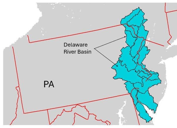
Figure 1a: Delaware River Basin.
 Figure 1b: Shows where the “Weather Data” button is located once you have completed the modeling step using the Watershed Multi-Year Model.
Land Cover
As described in Section 7.2.3, information on the type and areal extent of land use/cover within a given area of interest is extracted from the National Land Cover Dataset (NLCD 2019 or earlier) developed by the U.S. Geological Survey. Based on local information, however, a user may find that the land cover estimates provided via this approach may not accurately reflect the land use/cover distribution within a given area of interest (or they may wish to conduct “what if” analyses based on different land cover distributions). If so, the user can adjust the area values calculated from the NLCD data layer by using the “Land Cover” option associated with the “Add changes to this area” button shown in Figure 1b (above and the button is next to the Weather Data button).
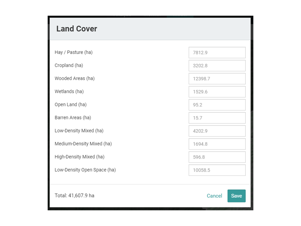
Upon selecting this option, the user is presented with a table like the one shown in Figure 2. At this point, the user can make changes by typing in new values for any of the categories shown. The user may make as many changes as desired, with the only requirement being that the new “Total” area must be equal to the initial total.
Conservation Practices
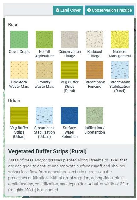
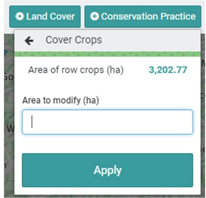
With the “Conservation Practice” option associated with the “Add changes to this area” tool in Model My Watershed, a user may simulate the potential load-reduction effects that might result from the implementation of a range of conservation practices (e.g., agricultural BMPs, urban storm-water BMPs, stream restoration activities, etc.). Upon initiating this option, the user is presented with a selection of practices from which to choose as shown in Figure 3. Upon selecting (i.e., clicking on) one of the practices, another window pops up that lets the user know how many units of measure (e.g., hectares, kilometers, etc.) are available for implementing the practice selected (see Figure 4). For example, in Figure 4, this window relays the information that 200.07 hectares of cropland are available for potential Cover Crop implementation in this particular watershed. In this case, the user would enter a value equal to or less than this number, and then click on the “Apply” button. Other practices can also be selected and “implemented” in a similar fashion.
Settings
Like most comprehensive simulation models, the GWLF-E model utilizes a wide range of parameters that effect the calculation of various hydrologic and pollutant load estimates provided as output. Summary descriptions of how values for many of these parameters are initially estimated are provided in Section 7.2.3 above. Within Model My Watershed, the user has the opportunity to edit some of the key parameter estimates via the “Add changes to this area” tool provided in Model My Watershed after an initial model run has been executed as shown in Figure 1. In this case, some of these key parameter values can be revised using the “Settings” option.
Once this particular option is initiated, the user is then presented with a series of tables (see Figure 5) that show the current calculated and default parameter values for the current model run. These can be changed by simply entering a new value and then clicking on the “Save” button at the bottom of each table. More information on how these values are calculated, and how they might reasonably be changed, is provided in the following sub-sections.
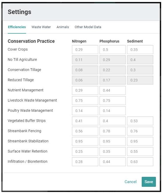
Efficiencies
The values provided in this table (see Figure 5) are the current BMP reduction coefficients used to simulate potential sediment, nitrogen, and phosphorus load reductions based on the implementation of a number of conservation practices or BMPs described earlier. These are primarily based on typical values found in the literature or as used by the USEPA in their Chesapeake Bay Watershed Model. New values can be entered by the user and applied to the next model run by clicking on the “Save” button located at the bottom of the window. These new values supplied by the user are presumed to be based on better locally-derived estimates of these coefficients. (Note that revisions to the “tillage-related” values are not currently allowed due to the complexity involved in calculating these coefficients within Model My Watershed. It is expected, however, that such changes will be allowed in future versions.)
Waste Water
Wastewater Treatment Plants
The estimated values for Wastewater Treatment Plants shown in Figure 6 (assuming they are non-zero) for Total Nitrogen, Total Phosphorus and Daily Effluent Discharge volume (in million gallons/day) are, by default, based on discharge data compiled by the USEPA (see related discussion in Section 7.2.3 above), and represent the total (summed) loads and/or volumes for one or more dischargers located within the area of interest (AoI). The values within any of these boxes shown in Figure 6 can be edited, and if so, should also represent the total loads and volume of all dischargers within the user-defined AoI.
In addition to directly editing the Total N, Total P and Volume (MGD) values in the appropriate boxes, users may also change point source loads by selecting one of two additional datasets provided in the pull-down menu. Note that if the AoI is inside the boundary of the Delaware River Basin, then all three point source dataset options are available (i.e., National EPA Data (NPDES), Updated PA Data (PADEP), and Updated Data from DRBC). However, for AoIs outside the DRB, only the first two options are available. Also, for AoIs outside the DRB, the National EPA Data (NPDES) dataset is used by default. Within the DRB, the Updated Data from DRBC is used by default. These other datasets are accessed by using the pull-down menu also shown in Figure 6.
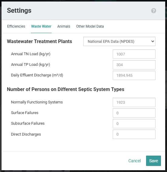
Figure 6: Shows the Waste Water tab within the Settings window that is accessed from the Settings button after an initial model run using the Watershed Multi-Year Model.
Number of Persons on Different Septic System Types
The values indicated for “normally functioning systems” are calculated in Model My Watershed using an estimate of the average number of persons per acre in “Low-Density Mixed” areas. In these areas, it is assumed that the populations therein are served by septic systems rather than centralized sewage systems. All homes in such areas are assumed to be connected to “normally functioning” systems rather than those that experience “surface breakouts” (surface failures), “short-circuiting” to underlying groundwater (subsurface failures), or have direct conduits to nearby water bodies. The values pertaining to any system type, however, can be adjusted by the user based on local information (see Fig. 6 above).
Animals
Animal Populations
As described earlier in Section 7.2.3, estimates of the number of farm animals contained within any given area are made using county-level census data on farm animal populations compiled by the U.S. Department of Agriculture. The calculated values for any given animal type, such as those shown in Figure 7, are only estimates, and may be updated with better local information on actual farm animal populations where possible. Within Model My Watershed, certain animals are automatically designated as “grazing” (e.g., dairy cows) or “non-grazing” (e.g., chickens), and these designations affect whether or not nutrient loads from such animals are deposited on pasture land or not. However, these designations can be changed by making the appropriate selection in the associated “pull-down” menu (i.e., “Yes” or “No”).
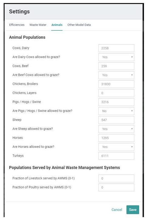
Populations Served by Animal Waste Management Systems
Animal Waste Management Systems (AWMSs) are designed for the proper handling, storage, and utilization of wastes generated from animal confinement operations, and typically include a means of collecting, scraping, or washing wastes from confinement areas into appropriate waste storage structures. Lagoons, ponds, or steel or concrete tanks are common structures used for the treatment and/or storage of liquid wastes, while storage sheds or pits are used to store solid wastes. Controlling runoff from roofs, feedlots, and “loafing” areas are also part of these systems. Adequate storage ensures wastes are only applied when crops can use the accompanying nutrients and soil and weather conditions are appropriate.
In this table, values from 0-1 are used to indicate the fraction of the total livestock population (e.g., cows, pigs, sheep, and horses) and/or the total poultry population (e.g., chickens and turkeys) that are believed to be served by AWMSs pertaining to each type in the area of interest. For example, if it is believed that the wastes from 35% of the livestock are treated by an AWMS, then a value of 0.35 would be entered in the appropriate cell. In the GWLF-E model, values greater than zero are used to calculate a reduction coefficient which is subsequently used to reduce nutrient loads from farm animal populations in the area of interest.
Other Model Data
Other model data, as shown in Figure 8, refers to estimated or default values set for various model parameters that affect the amounts of sediment, nitrogen and/or phosphorus that are generated within a given area of interest, and are subsequently transported and delivered to the outlet of that area. Within Model My Watershed, these parameter values are either calculated using various datasets (as described in Section 7.2.3 above), or based on typical values used in the literature.
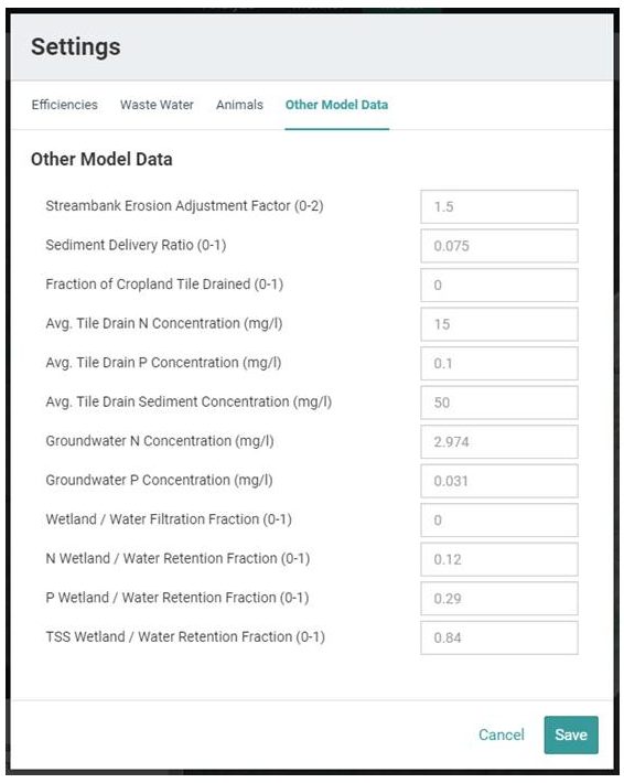
Streambank Erosion Adjustment Factor
Within Model My Watershed, the sediment and nutrient loads produced by eroding streambanks are estimated using an approach developed by Evans et al. (2003). This approach is based on a methodology often used in the field of geomorphology in which monthly streambank erosion is estimated by first calculating an average watershed-specific lateral erosion rate (LER) using the following equation:
LER = a * q0.6
where: LER = an estimated lateral erosion rate in meters/month
a = an empirically-derived constant related to the mass of soil eroded
from streambanks depending upon various watershed conditions, and
q = monthly stream flow in cubic meters per second.
Within Model My Watershed, after a value for LER has been computed, the total sediment load generated via streambank erosion is then calculated by multiplying the above erosion rate by the total length of streams in the watershed (in meters), the average streambank height (in meters), and an average soil bulk density value (in kg/m3). By adjusting the “streambank erosion factor” subsequent to a particular model run, one can increase or decrease the amount of streambank-eroded sediment, nitrogen and/or phosphorus simulated by GWLF-E. By default, this parameter value is set to “1.5” to account for the difference in the density of the stream network data layer used by Evan et al. (2003) in their original study and that of the NHD stream network used in Model My Watershed (in this case, the Model My Watershed stream layer is less dense than the other). As shown in Figure 8, users can increase this value up to 2, or decrease it to 0 (which would result in no streambank-generated loads).
Sediment Delivery Ratio
A sediment delivery ratio is based on the premise that a certain percentage of the material eroded from the land surface (usually the heavier soil particles) is deposited prior to reaching nearby water bodies. Empirically, the amount that does reach the outlet of a given watershed (called sediment yield) has been related to watershed size. Following the procedure described in Vanoni (1975), sediment delivery ratios calculated by Model My Watershed are based on the relationship:
SDR = 0.451(b-0.298)
where: SDR = sediment delivery ratio, and
b = size of the watershed in square kilometers.
After the initial model run, this particular parameter value can be adjusted to increase or decrease the amount of the internally-generated sediment load that is subsequently delivered to the watershed outlet. In this case, a value of 1 would imply that 100% of the generated sediment load would be delivered to the watershed outlet. Such cases are rare, however, since sediment delivery ratios for watersheds that range in size from about 10 to 1000 square kilometers (3.86 to 386 square miles) vary from about 0.15 to 0.05 when using the Vanoni method.
Fraction of Cropland Tile Drained
The GWLF-E model contains a relatively simple algorithm to account for the use of tile drains in agricultural areas of a watershed, as well as to estimate nutrient and sediment loads delivered by such systems. As shown in past studies completed in North America, water volumes in tile drains are typically about 40-60% of the total surface and subsurface runoff in agricultural landscapes with such systems (e.g., Tan et al., 2002 and Patni et al, 1996). Additionally, these and similar studies suggest that median values of nitrogen, phosphorus, and sediment concentration within tile drains are typically on the order of 15, 0.1, and 50 mg/l, respectively (e.g., Barry et al., 1993 and Fleming, 1990).
In GWLF-E, 50% of the surface and subsurface flow for each month based on weather inputs are re-distributed to tile drain flow in areas identified as being served by such systems. More specifically, tile drain flow for a watershed is estimated using information on the amount of cropland and the extent of tile-drained land in cropped areas. Information on the presence of cropland is extracted by Model My Watershed from the land use/cover layer, and information on the extent of tile-drained areas in a given watershed (i.e., “Fraction of Cropland Tile Drained”) is specified by the user.
Algorithmically, tile drain flow for a watershed is calculated using the equation:
TDF = 0.5 * CROPFLOW * FRACTILE
where: TDF = Total tile drain flow (in volume of water per month)
CROPFLOW = Total volume of surface and subsurface flow in cultivated
areas of the watershed per month
FRACTILE = Fraction of cultivated area that is tile-drained
Once the volume of tile drain water per month is calculated (in this case, liters of water), this volume is then multiplied by the “event mean concentrations” given above for nitrogen, phosphorus, and sediment (i.e., 15, 0.1, and 50 mg/l) to calculate loads for each in units of kg/mo. By default, the value for this parameter is “0”; however, the user can adjust this based on local information.
Average Tile Drain N Concentration
As indicated above, the default value for this parameter is 15 mg/l. However, the user may change it based on local knowledge or information.
Average Tile Drain P Concentration
As indicated above, the default value for this parameter is 0.1 mg/l. However, the user may change it based on local knowledge or information.
Groundwater N Concentration
An estimate of groundwater N concentration is used to calculate subsurface nitrogen loads delivered to the watershed outlet. As described in Section 7.2.3, this value is estimated based on the use of a national groundwater N concentration map previously developed by the USEPA. However, the user may wish to adjust this value based on more local knowledge or information.
Groundwater P Concentration
An estimate of groundwater P concentration is used to calculate subsurface phosphorus loads delivered to the watershed outlet. For use in GWLF-E, values for groundwater P concentration are estimated based on the use of a regression equation that relates groundwater P concentration to groundwater N concentration as calculated by Model My Watershed (and as described above). However, the user can adjust this value based on more local knowledge or information.
Wetland / Water Filtration Factor
In the GWLF-E model, a fairly simple attenuation routine has been implemented that allows the user to account for (i.e., approximate) the “pollutant-retention” effect of lakes, ponds and/or wetlands within the watershed being simulated. This tool is based on an empirical approach that reduces nutrient and sediment loads generated within the watershed using editable reduction coefficients and a user-specified estimate of the land area “drained” by such features. For example, in a watershed with the following conditions and settings:
- Initial (“pre-retention”) sediment load: 1000 kg/yr
- Percent of watershed area drained by wetlands/lakes/ponds: 60% (0.60)
- Sediment reduction coefficient: 0.88
the sediment load would be “re-calculated” as:
Re-calculated load after retention = (initial load of the drained area – (reduction coefficient x (initial load of the drained area)) + (percent area undrained x initial load)
= ((0.60 x 1000) – (0.88 x (0.60 x 1000))) + (0.40 x 1000)
= (600 – 528) + 400
= 472 kg/yr
As evident from the above discussion, the “retention” routine is fairly simple and is not intended to rigorously simulate the physical, chemical and biological processes that actually influence the transport of nutrients and sediment in watersheds where lakes, ponds and wetlands exist. However, this empirically-based approach does attempt to account for reduced loads that do occur as a result of these processes. In cases where such processes and reductions are significant, not accounting for them in some fashion may result in over-estimation of nutrient and sediment loads. In fact, in watersheds where many lakes, ponds and wetlands exist, it is highly likely that simulated pollutant loads will be significantly over-estimated unless attenuation is considered. Moreover, this problem typically becomes accentuated with very large watersheds (e.g., greater than the size of a typical HUC12 watershed, which has an average size of around 40 square miles in the conterminous U.S.).
In Model My Watershed, an option exists that allows users to invoke the attenuation (i.e., sub-basin modelling) routine for HUC10- and HUC8-size watersheds (see Figure 9 below). In this case, a value for a factor similar to the “wetland / water filtration factor” is automatically calculated using information on the extent of water and wetland acres that have already been derived by USGS for NHD catchments across the country (see Attributes for NHDPlus Catchments (Version 1.1) for the Conterminous United States: NLCD 2001 Land Use and Land Cover ). In cases where this factor has not been automatically calculated (e.g., with HUC12 basins or HUC10 and HUC8 basins where the “sub-basin modeling” option has not been used), the user has the ability to initiate the simple attenuation routine within GWLF-E by supplying a value between 0-1 for this parameter.
N Wetland / Water Retention Fraction
This factor indicates the typical fraction of the incoming nitrogen load to a wetland area or water body that is “retained” by these features. The default value of 0.12 is representative of the average value reported in the literature associated with the pollutant-reducing effects of such BMPs as constructed wetlands and storm-water retention/detention ponds. As with other parameters discussed above, this value can be changed by the user based on local knowledge or information.
P Wetland / Water Retention Fraction
This factor indicates the typical fraction of the incoming phosphorus load to a wetland area or water body that is “retained” by these features. The default value of 0.29 is representative of the average value reported in the literature associated with the pollutant-reducing effects of such BMPs as constructed wetlands and storm-water retention/detention ponds. As with other parameters discussed above, this value can be changed by the user based on local knowledge or information.
TSS Wetland / Water Retention Fraction
This factor indicates the typical fraction of the incoming TSS (sediment) load to a wetland area or water body that is “retained” by these features. The default value of 0.84 is representative of the average value reported in the literature associated with the pollutant-reducing effects of such BMPs as constructed wetlands and storm-water retention/detention ponds. As with other parameters discussed above, this value can be changed by the user based on local knowledge or information.
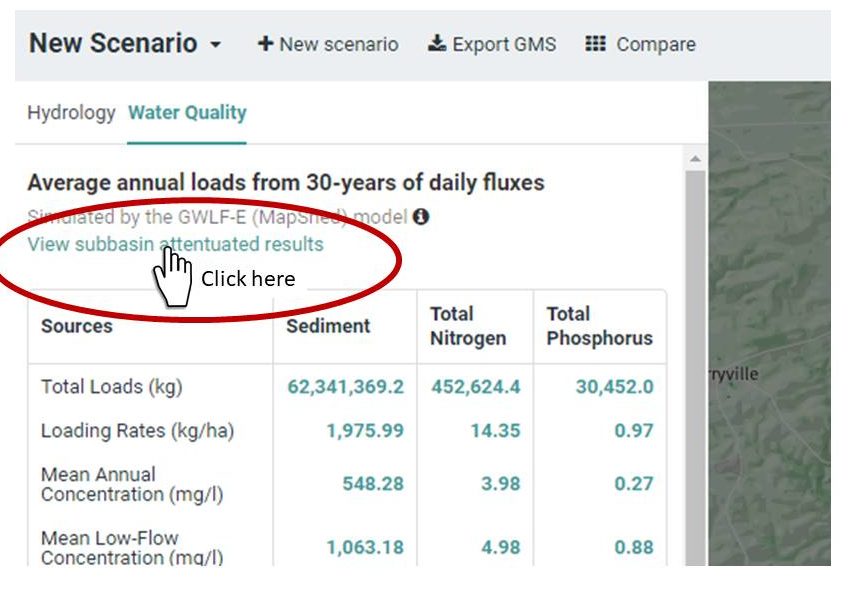
7.2.5 Subbasin Attenuated Results
Subbasin Modeling
In Model My Watershed, an option exists that allows users to invoke the attenuation (i.e., sub-basin modelling) routine for HUC12-, HUC10- and HUC8-size hydrologic units (see figure below). To access this tool you must:
- Select an area using “Select boundary” at either the USGS Subbasin unit (HUC-8), USGS Watershed unit (HUC-10), or USGS Subwatershed unit (HUC-12);
- Model your area using the Watershed Multi-Year Model;
- Click from the “Hydrology” tab to the “Water Quality” tab;
- Click on the “View subbasin attenuated results” text (in green near the top of the Average annual loads table (see Figure 10).
This subbasin modeling algorithm was developed by Scott Haag (Academy of Natural Sciences of Drexel University) and Barry Evans (Penn State University, ANS of Drexel, and Stroud Water Research Center) and was first released as the Stream Reach Assessment Tool (SRAT).
Stream Reach Assessment Tool Overview
The Stream Reach Assessment Tool (SRAT) was originally designed to integrate dozens of datasets to provide the following information specific to the Delaware River Basin:
- The mean annual pollutant load delivered to each of over 15,000 stream reaches in the Delaware River Basin from the immediate catchment of the stream reach. These loads are expressed as total loads (lbs/year) and loading rates (lbs/acre) for total nitrogen (TN), total phosphorous (TP) and total suspended sediment (TSS), and are segregated into each of the major sources affecting water quality (e.g., point sources, agriculture and urban/suburban runoff)
- The mean annual in-stream concentration (in mg/l) for each of the pollutants analyzed that aggregates pollutant loads from all upstream sources.
- Location and relative impact of point sources across the Basin.
Due to the influence of tides in coastal areas, it should be noted that SRAT estimates of TN, TP and TSS in these areas are not as accurate as they are in non-tidal areas due to the mixing of freshwater with estuarine and/or ocean waters which may significantly alter estimated pollutant concentrations.
As part of the SRAT development process, a limited amount of calibration was done to improve the overall accuracy of estimates produced using this approach. A more detailed explanation of this calibration is provided in SRAT Model Calibration.
SRAT Interpretation Assistance
Nitrogen and Phosphorus
High nutrient concentrations (particularly phosphorus in freshwater systems) can result in excessive plant growth (e.g., nuisance algae) and lower dissolved oxygen levels in streams. As a result, the level of nutrients in a stream is one good indicator of water quality.
In most fresh water bodies, phosphorus is the limiting nutrient for aquatic growth. Conversely, in most estuarine systems, nitrogen is the limiting nutrient. In some cases, however, the determination of which nutrient is the most limiting is difficult. For this reason, the ratio of the amount of N to the amount of P is often used to make this determination (Thomann and Mueller, 1987). If the N/P ratio is less than 10, nitrogen is limiting. If the N/P ratio is greater than 10, phosphorus is the limiting nutrient.
If the nutrient load to a water body can be reduced, the available pool of nutrients that can be utilized by plants and other organisms will be reduced and, in general, the total biomass can subsequently be decreased as well (Novotny and Olem, 1994). In most efforts to control eutrophication processes in water bodies, emphasis is placed on the limiting nutrient. This is not always the case, however. For example, if nitrogen is the limiting nutrient, it still may be more efficient to control phosphorus loads if the nitrogen originates from difficult to control sources such as nitrates in ground water.
Nutrient (i.e., nitrogen and phosphorus) loads primarily originate from wastewater treatment plants and agricultural land. Watersheds with high farm animal populations also tend to have higher nutrient loads. In this case, much of the animal waste is used as an organic fertilizer on surrounding cropland, which contributes to the nutrient loads emanating from these areas.
Sediment
With respect to stream health, high suspended sediment loads can reduce sunlight penetration through the water column, which may negatively impact various aquatic organisms. Such loads can also result in sediment build-up on the streambed that can degrade living conditions for benthic organisms. With respect to sources, sediment primarily originates from non-vegetated landscapes that are prone to surface erosion such as cropland. Streambank erosion is also a very important source of sediment, particularly in urbanized watersheds where the extent of impervious surface areas can lead to excessive “high-energy” runoff that can significantly erode streambanks during high-flow events. For the purposes of SRAT, simulated TSS (total suspended solids) estimates are for all practical purposes estimates of suspended sediment (TSS samples can include solids from other sources such as wastewater treatment plants; but these are considered to be negligible at the scale at which these analyses are done).
Pollutant Thresholds
Provided below is a table that presents some “threshold” values for nutrients and sediment that are intended to help determine whether a given watershed or stream segment might be impaired with respect to water quality. It must be understood, however, that these values are provided for guidance purposes only, and that actual impairments may vary based on many factors that interact at any given location. In the case of the values from Sheeder and Evans, both loading rate and in-stream concentration values are given. These latter values are to be interpreted as approximate “breakpoints” between impaired and unimpaired watersheds that were based on an analysis of observed stream data for 29 watersheds in Pennsylvania. The in-stream concentration values developed by USEPA and NJDEP, on the other hand, represent “targets” that each agency believes should be met to ensure unimpaired conditions within the general region of the Delaware River Basin. In the case of the USEPA values, a range is given for TN and TP due to that fact that values were developed for different ecoregions across the U.S, and the DRB covers two of these regions.
From the table, it can be seen that a threshold value of 0.1 mg/l seems appropriate for TP. Although the values range considerably for TN, it should be noted, as described earlier, that the value for TP is usually more important due to the fact that it is the limiting nutrient for most streams in the Delaware River Basin. In the case of TSS, NJDEP has set different threshold values for TSS depending upon whether the streams do or do not support trout.
Yields and Concentration Thresholds
| Source | TN | TP | TSS |
|---|---|---|---|
| Sheeder and Evans | 13.0 kg/ha (14.6 lb/ac) | 0.30 kg/ha (0.34 lb/ac) | 785 kg/ha (882 lb/ac) |
| Sheeder and Evans | 3.0 mg/L | 0.07 mg/L | 197 mg/L |
| USEPA | 0.07-1.0 mg/L | 0.006-0.1 mg/L | — |
| NJDEP | 10.0 mg/L | 0.1 mg/L | 25-40 mg/L (trout vs. non-trout) |
*Note the actual nitrogen values given in Sheeder and Evans are for inorganic N only and are lower than those shown in the table above. The values shown above have been adjusted upwards to account for organic N as well. Also note that the TN values for NJDEP are for nitrate-N only. In this case, the value appears to be based on the national 10 mg/L drinking water standard rather than ecological or nutrient enrichment factors.
Sources:
Novotny, V., and H. Olem. 1994. Water Quality: Prevention, Identification, and Management of Diffuse Pollution. Van Nostrand Reinhold, New York.
Thomann, R.V., and J.A. Mueller. 1987. Principles of Surface Water Quality Modeling and Control. Harper & Row, New York.
Sheeder, S.A., and Evans, B.M. 2004. Estimating nutrient and sediment threshold criteria for biological impairment in Pennsylvania watersheds. J. Am.Water Res. Assoc. 40, 881–888.
7.2.6 Model Calibration
Overview
As described elsewhere in the technical documentation for Model My Watershed, there are two basic modelling approaches included in this tool. The simpler model provides pollutant load estimates based on literature-based “event mean concentrations” and user-supplied rainfall values. The other more comprehensive “multi-year” model is based on the MapShed desktop software application developed by Dr. Barry Evans and his group at Penn State University (Evans and Corradini, 2016). The MapShed model itself includes a GIS-based front-end for assembling input data for an enhanced version of the GWLF model originally developed by Haith and Shoemaker (1987). This enhanced model (called GWLF-E) is the model upon which the “multi-year” model included in Model My Watershed is based.
To provide a preliminary assessment of the accuracy of the multi-year model, a limited amount of calibration was performed using modeled results and observed stream data for 39 test watersheds located in specific geographic regions located around the country. Due to a lack of time initially assigned to this particular task under current Model My Watershed funding, the limited calibration was undertaken using stream data and load calculations previously compiled by one of the lead modelers involved in the development of the “multi-year” model included in the Model My Watershed application (i.e., Dr. Evans) as part of other projects that he has conducted over the last 15 years or so (e.g., Evans et al., 2002; Evans, 2007; and Evans, 2010).
As part of these earlier projects, daily stream flow and water quality data were obtained from USGS National Water Information System, and daily and/or monthly pollutant loads for calibration periods ranging from about 1990 to 2015 were subsequently computed for each corresponding drainage area using a variety of statistical methods (primarily the FLUX model from the U.S. Army Corps of Engineers [Walker, 1999]). For the purposes of the current assessment, loads previously computed in this fashion were then used as the “observed” loads against which Model My Watershed-simulated loads were compared. Figure 11 depicts the distribution of these different test sites across the country, and Table 1 summarizes the size, pollutant loads, and original calibration periods associated with each of these sites.
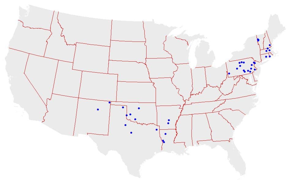
Table 1. Summary Data for Calibration Test Sites
| Test Site | Location | Size (sq km) | Total Nitrogen | Total Phosporus | Sediment | Original Calibration Period |
|---|---|---|---|---|---|---|
| Bayou Annacoco | LA | 995 | X | 1997-2006 | ||
| Bayou Toro | LA | 357 | X | X | 1997-2006 | |
| Beech Creek | PA | 444 | X | X | 1990-1996 | |
| Big Sandy Creek | TX | 749 | X | X | 1997-2006 | |
| Black Cypress Creek | TX | 925 | X | X | 1997-2006 | |
| Bushkill Creek | PA | 303 | X | X | X | 1989-1999 |
| Carrizozo Creek | NM | 505 | X | X | X | 1997-2006 |
| Chartiers Creek | PA | 712 | X | X | 1990-2006 | |
| Chiques Creek | PA | 280 | X | X | X | 2002-2014 |
| Clearfield Creek | PA | 977 | X | X | 1990-1996 | |
| East Cache Creek | OK | 1787 | X | X | X | 1997-2006 |
| Elk Creek | OK | 1430 | X | X | 1997-2006 | |
| Elm Fork/North Fork | TX/OK | 2178 | X | X | X | 1997-2006 |
| Gallinas Creek | NM | 759 | X | X | X | 1997-2006 |
| Hurricane Creek | AR | 510 | X | X | X | 1997-2006 |
| Kettle Creek | PA | 638 | X | X | X | 1990-1996 |
| Lamprey River | NH | 474 | X | X | X | 1997-2004 |
| Laplatte River | VT | 114 | X | X | 1997-2004 | |
| Lehigh River | PA | 3520 | X | X | X | 1989-1999 |
| Lewis Creek | VT | 199 | X | X | X | 1997-2004 |
| Little Otter Creek | VT | 148 | X | X | X | 1997-2004 |
| Lycoming Creek | PA | 558 | X | X | X | 1990-1996 |
| Moro Creek | AR | 997 | X | X | X | 1997-2006 |
| Paulins Kill | NJ | 326 | X | X | X | 2006-2015 |
| Pawcatuck Creek | CT/RI | 764 | X | X | 1997-2004 | |
| Pequea Creak | PA | 397 | X | 1989-1999 | ||
| Pine Creek | PA | 2552 | X | X | X | 1990-1996 |
| Saline Bayou | LA | 653 | X | X | 1997-2006 | |
| Salmon River | CT | 259 | X | X | 1997-2004 | |
| Schuylkill River | PA | 4903 | X | X | 1990-1996 | |
| Sherman Creek | PA | 633 | X | X | X | 1990-1996 |
| Skeleton Creek | OK | 1026 | X | X | 1997-2006 | |
| South Fork Wichita River | TX | 1479 | X | X | X | 1997-2006 |
| Squannacook River | MA/NH | 171 | X | X | X | 1997-2004 |
| Sudbury River | MA | 275 | X | X | 1997-2004 | |
| Ware River | MA | 249 | X | 1997-2004 | ||
| Wissahickon Creek | PA | 165 | X | 1989-1999 | ||
| Wolf Creek | TX | 2038 | X | X | X | 1997-2006 |
| Yellow Breeches Creek | PA | 566 | X | X | 1990-1996 | |
| Total Sites | 35 | 34 | 25 |
Model Results and Discussion
As described above, Model My Watershed was used to estimate nutrient and sediment loads for each of the calibration test sites. As part of the calibration process, the loads delivered to the outlet of the drainage areas represented by the calibration test sites were calculated and subsequently compared to the observed loads at each outlet. With the new attenuation routine implemented in Model My Watershed, nutrient and sediment loads are attenuated (i.e., reduced) as the loads move from upstream NHD catchments to downstream NHD catchments based on the presence (percent) of open water and wetland areas within each intervening catchment down to the drainage area outlet. During the calibration process, the attenuation rates were incrementally adjusted in successive model runs until a “best fit” was achieved across all of the test sites in terms of matching observed and simulated loads. Table 2 shows these loads (expressed as loading rates in kg/ha) for each of the calibration sites.
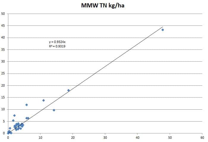
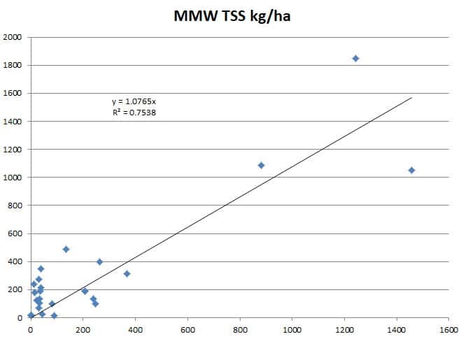
Figures 2 through 4 graphically show the comparisons between the observed and simulated loads for the calibration points using the mean annual loading rate (in kg/ha) as a standardized unit of measure. As can be seen from these figures, the Model My Watershed model simulations provided reasonably good estimates of the total nitrogen and total phosphorus loads on a mean annual basis (i.e., R2 = 0.93 and R2 = 0.83, respectively). In the case of total suspended sediment (TSS) loads, the model results were less accurate (R2 = 0.75).
As can be seen for TN, estimates from Model My Watershed were under-predicting loads by about 7% on average. In this case, it is suspected that the under-prediction may be due, in part, to the general unavailability of good data on nitrogen discharges from wastewater treatment plants across the country. In Model My Watershed, data from the USEPA is used to estimate nitrogen loads from these sources. However, in many states only ammonia concentrations (which are general a very small fraction of TN) are typically required by regulatory agencies and subsequently reported to EPA.
Additionally, in Model My Watershed, county-level data on farm animal populations from USDA are used to estimate animal numbers for any given watershed or area of interest based on an area-weighted basis (i.e., area of agricultural land). It is highly unlikely, though, that farm animal populations are as uniformly distributed as this algorithm implies. In general, the problem of under-estimating TN appears to worsen in watersheds having very large TN loading rates (e.g., higher than about 10 kg/ha). For example, in two of the test sites used in Pennsylvania (i.e., Lehigh River and Chiques Creek), it is known that the farm animal populations and/or TN loads from wastewater discharges are higher than those estimated by Model My Watershed based on locally-available data.
Table 2. Comparison of Observed and Simulated Loads for the Calibration Sites
| Bayou Annacoco | 3.85 | NA | NA | 1.96 | NA | NA |
| Bayou Toro | 4.61 | 0.72 | NA | 3.44 | 0.22 | NA |
| Beech Creek | 1.58 | 0.12 | NA | 5.35 | 0.20 | NA |
| Big Sandy Creek | 0.11 | NA | 30.7 | 0.63 | NA | 71.3 |
| Black Cypress Creek | NA | 0.26 | 23.2 | NA | 0.24 | 124.5 |
| Bushkill Creek | 2.51 | 0.15 | 34.0 | 1.50 | 0.07 | 106.2 |
| Carrizozo Creek | 0.02 | 0.004 | 0.9 | 0.07 | 0.01 | 14.1 |
| Chartiers Creek | 6.17 | 0.58 | NA | 6.29 | 1.18 | NA |
| Chiques Creek | 47.80 | 2.32 | 881.5 | 43.36 | 2.71 | 1085.4 |
| Clearfield Creek | 4.34 | 0.22 | NA | 2.92 | 0.31 | NA |
| East Cache Creek | 2.10 | 0.49 | 263.4 | 2.67 | 0.23 | 400.5 |
| Elk Creek | 2.10 | 0.23 | NA | 3.17 | 0.24 | NA |
| Elm Fork / North Fork | 0.40 | 0.07 | 33.6 | 0.87 | 0.09 | 132.2 |
| Gallinas Creek | 1.0 | 0.17 | 89.0 | 0.12 | 0.01 | 14.3 |
| Hurricane Creek | 2.45 | 0.26 | 37.3 | 1.95 | 0.11 | 214.8 |
| Kettle Creek | 3.25 | 0.13 | 248.0 | 2.27 | 0.16 | 97.8 |
| Lamprey River | 0.60 | 0.17 | 14.6 | 2.08 | 0.12 | 181.2 |
| Laplatte River | 3.30 | 0.75 | NA | 2.31 | 0.50 | NA |
| Lehigh River | 14.16 | 0.73 | 133.9 | 9.75 | 1.08 | 488.9 |
| Lewis Creek | 3.29 | 0.39 | 81.6 | 2.94 | 0.34 | 97.9 |
| Little Otter Creek | 3.91 | 0.62 | 207 | 3.35 | 0.56 | 188.3 |
| Lycoming Creek | 3.26 | 0.13 | 206.0 | 3.80 | 0.29 | 188 |
| Moro Creek | 3.06 | 0.27 | 37.1 | 1.82 | 0.06 | 191 |
| Paulins Kill | 5.72 | 0.20 | 37.7 | 6.39 | 0.38 | 346.6 |
| Pawcatuck Creek | 1.96 | NA | 30.3 | 7.45 | NA | 272.1 |
| Pequea Creek | NA | NA | 1458.0 | NA | NA | 1050.8 |
| Pine Creek | 3.18 | 0.19 | 238.0 | 4.14 | 0.29 | 136.4 |
| Saline Bayou | 2.37 | 0.25 | NA | 2.72 | 0.12 | NA |
| Salmon River | 2.55 | 0.08 | NA | 3.33 | 0.24 | NA |
| Schuylkill River | 18.72 | 1.33 | NA | 17.99 | 1.94 | NA |
| Sherman Creek | 5.73 | 0.20 | 368.0 | 11.96 | 0.65 | 315.3 |
| Skeleton Creek | 4.23 | 0.23 | NA | 3.96 | 0.30 | NA |
| South Fork Wichita River | 0.69 | 0.27 | 43.4 | 0.27 | 0.03 | 22.8 |
| Squannacook River | 2.58 | 0.17 | 11.6 | 3.82 | 0.15 | 236.8 |
| Sudbury River | 2.88 | 0.21 | NA | 3.78 | 0.35 | NA |
| Ware River | NA | 0.14 | NA | NA | 0.19 | NA |
| Wissahickon Creek | NA | NA | 1242.0 | NA | NA | 1849 |
| Wolf Creek | 0.21 | 0.003 | 0.3 | 0.25 | 0.03 | 18.1 |
| Yellow Breeches Creek | 10.94 | 0.40 | NA | 13.77 | 0.81 | NA |
NA – In-stream sample data not available.
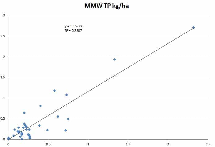
In the case of TP, Model My Watershed-predicted loads were about 16% higher on average than observed loads. Also, as shown by the lower R2 value (0.83), Model My Watershed was less accurate in predicting these loads than TN, particularly in cases where lower loading rates occurred (below about 1 kg/ha). As with TN, it may be that inaccurate estimates of wastewater discharges and farm animal populations are adversely influencing TP load estimates from Model My Watershed. Since much of the phosphorus load generated within a given watershed is also attached to stream-transported sediment, however, it is also possible that inaccurate estimates of sediment loads (as discussed below) are also adversely affecting these load estimates.
As shown in Figure 4, sediment loads predicted by Model My Watershed are about 8% higher than observed loads on average, and the R2 value (0.75) is lower than that for either TN or TP. This is not surprising as in-stream samples of sediment are known to be very problematic, and it could be that some of the inaccuracy in the modeled results comes from the use of imprecisely-calculated “observed” values. It is also likely that prediction errors may be arising due to the more “empirical” nature of the streambank erosion routine in the GWLF-E model in comparison to those used for calculating sediment erosion from upland sources. However, it is hoped that future improvements in this routine that allow for better distribution of streambank-eroded loads on a stream segment basis (rather than the more “uniform” approach used now) will improve these results. In any case, it is believed that the simulation results do capture the relative magnitudes of sediment loads in streams that are relatively “natural” versus those heavily influenced by agriculture and human development reasonably well.
As described earlier, only a limited amount of calibration could be performed due to a lack of funding to accomplish this activity in the original scope of work. However, with future funding, it is anticipated that additional calibration work will be completed. In particular, as implied by the map in Figure 11, additional work needs to be undertaken in other regions of the country that have different weather patterns, landscape conditions, cropping practices, etc. from those reflected by the locations of existing test sites used for this limited calibration in order to provide a higher level of confidence in the pollutant loading estimates produced by Model My Watershed elsewhere across the country. For those so inclined, Model My Watershed currently provides the ability to download an input (gms) file generated for any given watershed or area of interest. Once downloaded, this file can be read by the desktop version of the GWLF-E model and then subsequently edited to support other calibration efforts.
References Cited
- Evans, B.M., D.W. Lehning, K.J. Corradini, G.W. Petersen, E. Nizeyimana, J.M. Hamlett, P.D. Robillard, and R.L. Day. 2002. A comprehensive GIS-based modelling approach for predicting nutrient loads in watersheds. J. Spatial Hydrology 2(2).
- Evans, B.M. 2007. Summary of Work Undertaken Related to Adaptation of AVGWLF for Use in New England and New York. Final Report to the New England Interstate Water Pollution Control Commission, Penn State Institutes of Energy and the Environment, 116 pp.
- Evans, B.M. 2010. Adaptation of the AVGWLF Watershed Model for Use in Texas and Surrounding States: Phase 1. Report to the Texas State Soil and Water Conservation Board, Penn State Institutes of Energy and the Environment, 157 pp.
- Evans, B.M., and K.J. Corradini. 2016. MapShed Users Guide (Version 1.5), Penn State Institutes of Energy and the Environment, Penn State University, 140 pp.
- Haith, D.A., and L.L. Shoemaker. 1987. Generalized Watershed Loading Functions for Stream Flow Nutrients. Water Resources Bulletin, 23(3), pp. 471-478.
- Walker, W. W. 1999. Simplified Procedures for Eutrophication Assessment and Prediction: User Manual. Prepared for U.S. Army Corps of Engineers, Instruction Report W-96-2, 239 pp.
7.3 Watershed Multi-Year Worksheet
Watershed Multi-Year Model for Analysis of Sub-Area Within a Larger HUC12
This particular tool was created to meet the needs of users in Pennsylvania that are conducting watershed modeling activities related to the development of a Pollution Reduction Plan (PRP) as part of an NPDES permit renewal for regulated areas that are responsible for managing urban stormwater runoff.
In developing a PRP, an analysis of the pollutant load contributed by a smaller area (typically, a municipality or similar urbanized area) within a larger watershed (in this case, a HUC12 basin) must be completed. After the loads for the “urbanized” area have been established, an analysis must then be conducted to estimate the potential load reduction that might be achieved via the implementation of various stormwater control measures.
Currently, sediment load reductions of 10% from existing loads are required in Pennsylvania. Although this tool is geared towards users in Pennsylvania, its application to similar problems in other areas outside of Pennsylvania are certainly possible.
With this tool, users are required to identify the smaller area of interest (AoI) such as a municipality, urban planning area, etc. using one of three options provided in Model My Watershed as described in Sections 7.2 through 7.4 above (i.e., “Draw Area”, “Delineate Watershed” or “Upload File”).
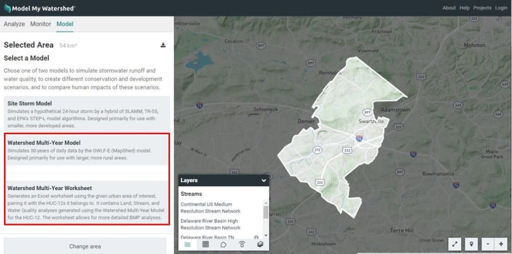
Once this area has been defined, the user must then select the second (lower) of the two Watershed Multi-Year Model options shown in Figure 15 to simulate hydrology and pollutant loads for the AoI. With the first (upper) option, the model is only used to generate hydrology and pollutant load output for a single, selected AoI. With the second (lower) option, however, land cover distribution and pollutant load data are automatically written to an Excel-formatted “BMP Spreadsheet Tool” that is subsequently made available for download to the user.
With this latter BMP tool, it is possible for users to conduct a wider range of load reduction scenarios than is possible using the more stream-lined “Conservation Practices” option described in Section 7.2.4. With this tool, the HUC12 basin within which the specified AoI is located is automatically identified. Also, if the AoI spans more than one HUC12 basin, additional BMP spreadsheets are filled out based on land cover data and load estimates for each HUC12 basin, and then made available for download by the user automatically.
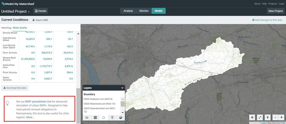
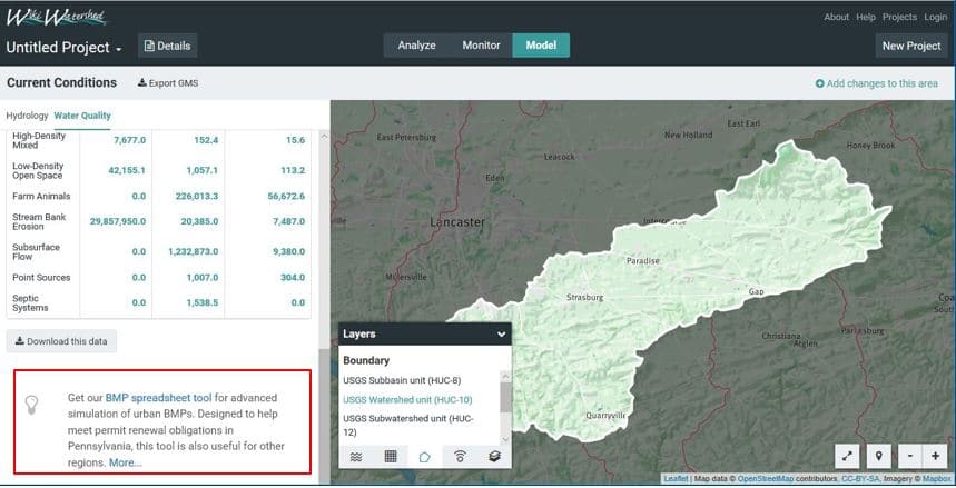
The BMP Spreadsheet Tool described above was made available in previous versions of Model My Watershed, and can also be accessed by clicking on the appropriate link on the Water Quality output tab as shown in Figure 16 below if the first (upper) Watershed Multi-Year Model option shown in Figure 15 is selected. In this case, however, the Excel-formatted spreadsheet that is made available for download does not have land cover data and model results automatically entered as described above. Rather, the user must copy and paste this information manually as described in the user manual that can also be downloaded below.
Also included in this manual are instructions on how to use the spreadsheet tool for conducting various BMP scenarios once the required land cover and load data have been entered either manually or automatically as described in this subsection. Copies of a blank spreadsheet tool and one filled in with sample data can be downloaded below.
- Model My Watershed BMP Spreadsheet Tool User Manual
- Model My Watershed BMP Spreadsheet Tool (blank)
- Model My Watershed BMP Spreadsheet Tool (example)
Note: if you are unable to see the link to download the Watershed Multi-Year Worksheet, you may need to use the scroll bar on the left panel or the zoom out feature in your browser settings.
